Raj Narayan Dhara, Ph.D. Applied Mathematics

INTRODUCTION

Differential equations are equations involving derivatives of functions. Derivative describes the rate of change of the given function at a given moment.

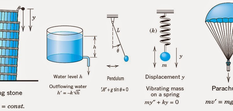
Differential equations have been around for almost as long as derivatives. Once people started calculating derivatives and applying them to real-world problems, they quickly realized the immense value of reversing the process. Instead of finding the derivative of a known function, it became crucial to determine the function based on the differential equations that its derivatives must satisfy. For instance, when an object is in motion, the rate at which its position changes over time is called its velocity. It shows how the position of the object changes as time passes. On the other hand, the object’s acceleration is determined by the second derivative of its position with respect to time. This tells us how the velocity of the object changes as time progresses.

These equations, known as ordinary differential equations (ODEs), involve functions that depend on a single variable, often time. On the other hand, partial differential equations (PDEs) are more versatile as they involve functions that depend on multiple variables, like several spatial variables or functions of both space and time.

Exploring the Boundless Applications of Differential Equations

Differential equations, with their elegant yet formidable nature, serve as the bedrock upon which a vast array of scientific and engineering endeavors stand. From deciphering the celestial movements of planets to designing resilient bridges and understanding the intricate workings of biological systems, the applications of these mathematical constructs are as diverse as they are profound.

1. Population Growth: Differential equations can model the growth and decline of populations over time. For example, the logistic equation is commonly used to describe population growth with limited resources. The graph of this equation shows how the population reaches a carrying capacity, leveling off as it approaches the maximum sustainable size.
2. Heat Diffusion: Differential equations are used to model the spread of heat in various materials. The heat equation describes how temperature changes over time and space. Visualizations of heat diffusion can show how temperature gradients evolve and how heat spreads through different materials.
3. Fluid Flow: Fluid dynamics relies heavily on differential equations to describe the behavior of liquids and gases. The Navier-Stokes equations are a set of differential equations that govern fluid flow. Visualizations of fluid flow phenomena, such as water flowing through pipes or air currents around objects, can be generated based on these equations.
4. Electrical Circuits: Electrical engineers use differential equations to study and design circuits. For instance, the differential equations for a simple resistor-capacitor (RC) circuit can be used to analyze how charge and voltage change over time. Visualizations can show how electrical signals evolve and how components interact within a circuit.
5. Wave Propagation: Differential equations are instrumental in understanding the behavior of waves, such as sound waves or electromagnetic waves. The wave equation describes the propagation of waves through space and time. Visualizations can demonstrate wave phenomena like interference, diffraction, and standing waves.
6. Neural Network Training: Differential equations come into play when training neural networks. One common approach is to use gradient-based optimization algorithms, such as stochastic gradient descent (SGD). These algorithms utilize the gradients of the network’s parameters with respect to the loss function, which are essentially partial derivatives, to update the network’s weights and biases during the training process.
7. Reinforcement Learning: Differential equations find applications in reinforcement learning algorithms, which involve an agent learning to make sequential decisions based on feedback from its environment. Techniques like the Hamilton-Jacobi-Bellman equation and the Pontryagin’s minimum principle are employed to solve optimal control problems in reinforcement learning, allowing the agent to learn and optimize its decision-making process.
8. Time-Series Analysis: Differential equations are valuable for analyzing and modeling time-series data, which involve observations taken at different points in time. Techniques like autoregressive integrated moving average (ARIMA) models and stochastic differential equations (SDEs) are used to model and predict the behavior of time-series data, making them useful in various AI and ML applications, such as stock market forecasting and weather prediction.
9. Physics-Informed Machine Learning: Differential equations are integrated with machine learning techniques to incorporate physical laws and constraints into AI models. This approach, known as physics-informed machine learning, combines data-driven learning with the governing equations of a system. By incorporating differential equations as constraints or regularization terms, it allows models to capture both data patterns and physical principles, leading to more robust and accurate predictions.

These are just a few examples of how differential equations intersect with AI and ML. They provide a mathematical foundation for understanding and improving the algorithms and techniques used in these fields, allowing us to tackle complex problems and make predictions based on observed data.

Problem with modeling?

If your studies or company need assistance related to differential equations and various aspects of mathematical modeling with it, feel free to discuss your project in more detail. We’re here to help!

REFERENCES

1. Boyce, W.; DiPrima, R.; Meade, D. (2017). Elementary Differential Equations and Boundary Value Problems. Wiley.
2. Coddington, E. A.; Levinson, N. (1955). Theory of Ordinary Differential Equations. McGraw-Hill.
3. Goodfellow, I., Bengio, Y., & Courville, A. (2016). Deep Learning. MIT Press.
4. Box, G. E., Jenkins, G. M., & Reinsel, G. C. (2015). Time Series Analysis: Forecasting and Control. Wiley.
5. Brunton, S. L., & Kutz, J. N. (2019). Data-Driven Science and Engineering: Machine Learning, Dynamical Systems, and Control. Cambridge University Press.